Alt text

machisplin

An R package for interpolation of noisy multi-variate data through comprehensive statistical analyses using thin-plate-smoothing splines and machine learning ensembling. This package is a free open-source machine learning analog to the expensive ANUSPLIN software.

To install, open R and type the following:

install.packages("devtools")
library(devtools)
install_github("jasonleebrown/machisplin")

Contact

We can help you sort out issues, maybe

Input Data formats

To explore data format for input data, see:

library(raster)
library(MACHISPLIN)
##data format that will be interpolated, each column is a different dataset
Mydata<-sampling

#rasters to use as high resolution co-variates for downscaling
ALT = raster(system.file("extdata", "alt.tif", package="MACHISPLIN"))
SLOPE = raster(system.file("extdata", "slope.tif", package="MACHISPLIN"))
TWI = raster(system.file("extdata", "TWI.tif", package="MACHISPLIN"))

If needed, see guide below to convert raster GIS data for use as in ‘MACHISPLIN’

What does it do?

This R package interpolates noisy multi-variate data through machine learning* ensembling of up to six algorithms: boosted regression trees (BRT), neural networks (NN); generalized additive model (GAM), multivariate adaptive regression splines (MARS), support vector machines (SVM), and random forests (RF). The machisplin.mltps function simultaneously evaluates different combinations of the six algorithms to predict the input data. During model tuning, each algorithm is systematically weighted from 0-1 and the fit of the ensembled model is evaluated. The best performing model is determined through k-fold cross validation (k=10) and the model that has the lowest residual sum of squares of test data is chosen. After determining the best model algorithms and weights, a final model is created using the full training dataset. Residuals of the final model are calculated from the full training dataset and these values interpolated using thin-plate-smoothing splines. This creates a continuous error surface and is used to correct most the residual error in the final ensemble model.

This package is a free open-source machine learning analog to the expensive ANUSPLIN software. To output final R2 values, model weights, algorithm(s) used, and rasters for use in GIS; use the machisplin.write.geotiff function. To output residuals use machisplin.write.residuals and to output model loadings use machispline.write.loadings. *just to clarify, GAMs are not a machine learning method

Alt text Overview of process

Alt text Details of modeling using higher resolution covariates

Alt text Example of the results (all with R2>0.99).

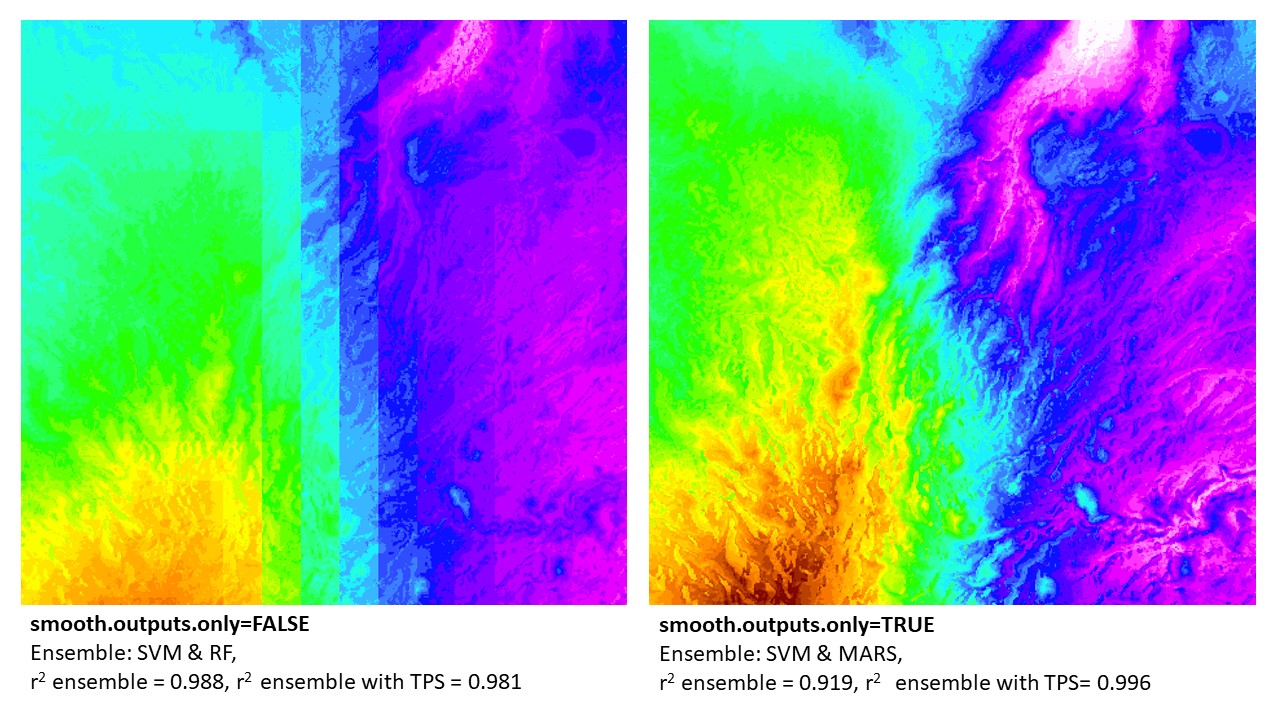
Update: New Parameter (1/15/2021): smooth.outputs.only

I recently added a new parameter ‘smooth.outputs.only’ to the machisplin.mltps function to address an issue with occasionally blocky results. If ‘smooth.outputs.only=TRUE’, this removes Boosted Regressive Trees and Random Forests from the modeling algorithms. Both algorithms occasionally produce blocky outputs (see example below). I recommend first using ‘smooth.outputs.only=FALSE’ for the initial analyses. If you are unhappy with the visual appearance of the created layers, consider ‘smooth.outputs.only=TRUE’. Be aware if results are blocky and you exclude these two algorithms, then the predictive performance might decline (as before exclusion, one or both contributed to the best model).

My biggest concern with blocky interpolated surfaces, in addition to looking bad, is the blockiness itself might be the result of overfitting to noise in the training datasets. In most cases, I think smooth continuous surfaces best characterize most spatial processes. Thus, smoother results might better represent the truth, despite slightly lower performances values.

Alt text BIO13 downscaled in northern Madagascar: example of ‘smooth.outputs.only’ parameter. Note that the final results that are merged with thin-plate-splines (TPS) error surfaces were better using the ‘smooth.outputs.only=TRUE’ (vs. ‘smooth.outputs.only=FALSE’). In this case, the TPS could better ‘fix’ the ‘smooth.outputs.only=TRUE’ ensemble models. In contrast, the ‘smooth.outputs.only=FALSE’ ensemble models (without TPS) had a higher r2. This can be due to the TPS not able to correct error in blocky models. In this example (and all where r2 ensemble > r2 ensemble + TPS), the final model produced was the r2 ensemble (w/o TPS). However, in all cases, the raw ensemble of ‘smooth.outputs.only=FALSE’ will always be lower than, or equal to, the model run with ‘smooth.outputs.only=TRUE’.

Example 1 - using provided datasets

library(MACHISPLIN)
library(raster)

##load spatial data with (coordinates named exactly as 'long' and 'lat') and any number of layers to downscale
##note this can be from a raster of lower resolution climate data or point weather station data
data(sampling)
Mydata<-sampling

#load rasters to use as high resolution co-variates for downscaling
ALT = raster(system.file("extdata", "alt.tif", package="MACHISPLIN"))
SLOPE = raster(system.file("extdata", "slope.tif", package="MACHISPLIN"))
TWI = raster(system.file("extdata", "TWI.tif", package="MACHISPLIN"))

# function input: raster brick of covarites
raster_stack<-stack(ALT,SLOPE,TWI)

#run an ensemble machine learning thin plate spline 
interp.rast<-machisplin.mltps(int.values=Mydata, covar.ras=raster_stack, smooth.outputs.only=FALSE, n.cores=2)

machisplin.write.geotiff(mltps.in=interp.rast)
machisplin.write.residuals(mltps.in=interp.rast)
machisplin.write.loadings(mltps.in=interp.rast)

Example 2 - typical workflow

see below for help formating raster/environment data.

library(MACHISPLIN)
library(raster)

# Import a csv as shapefile:
Mydata<-read.delim("sampling.csv", sep=",", h=T)

#load rasters to use as high resolution co-variates for downscaling
ALT = raster("SRTM30m.tif")
SLOPE = raster("ln_slope.tif")
TWI = raster("TWI.tif")

# function input: raster brick of covarites
raster_stack<-stack(ALT,SLOPE,TWI)

#run an ensemble machine learning thin plate spline 
interp.rast<-machisplin.mltps(int.values=Mydata, covar.ras=raster_stack, smooth.outputs.only=TRUE, n.cores=2, tps=FALSE)

#to plot results (change number to select different output raster)
plot(interp.rast[[1]]$final)

#to view residuals (change number to select different output raster)
interp.rast[[1]]$residuals

#to view model loadings
interp.rast[[1]]$var.imp

#to view other model parameters and other parameters
interp.rast[[1]]$summary

Getting environmental data formatted for ‘MACHISPLIN’

You need two sets of datafiles. 1. the layers that will be interpolated and 2. higher resolution covariates that will be use to downscale interpolation layers.

1. Layers to be interpoloated

This is a single data file where the first two columns are longitude and latitude (x and y) in that order. The following columns represent the corresponding values of the data layers that will be interpoloated. This can a single layer (=1 column) or a dozen (=12 columns). These values can be obtained from field data (e.g. weather station measurements) or directly from a lower resolution raster.

2. High-resolution covariates

These need to be a series of high resolution raster combinded into a raster stack. All rasters must be the same: resolution, projection and extent. Typically these are microtopgraphic layers.

Importing rasters into R

library(raster)

##rasters to downscale (= make higher resolution), here they 'Tiff' rasters are in base working directory
BIO1 = raster("bio1.tif")
BIO2 = raster("bio2.tif")
BIO12 = raster("bio12.tif")
BIO15= raster("bio15.tif")

##high-resolution covariate rasters
ALT = raster("SRTM30m.tif")
SLOPE = raster("ln_slope.tif")
TWI = raster("TWI.tif")

Clipping the extent of rasters in R

##create raster stack to speed process up 
raster_interp_layers<-stack(BIO1, BIO2, BIO12, BIO15)
raster_covar_layers<-stack(ALT, SLOPE, TWI)

##define extent for which you will clip data to. These values will reflect the spatial area of analyses and the area where you will create high resolution variables.    
##I highly recommend determining these values from a GIS (ArcGIS or Google Earth).
##extent order input below is: xmin, xmax, ymin, yma
e.in <- extent(-160, 10, 30, 60)

##perform crop function to clip to input extent
interp_layers <- crop(raster_interp_layers, e.in)	
covar_layers <- crop(raster_covar_layers, e.in)	

Convert input ‘rasters to be interpolated’ to ‘MACHISPLIN’ format (continued from previous step)

##convert one of the rasters to a point dataframe to sample.  Use any raster input.
env.points<-rasterToPoints(BIO1, fun=NULL, spatial=FALSE)

##subset only the x and y data
env.points<- env.points[,1:2]

##Extract values to points from rasters
RAST_VAL<-data.frame(extract(interp_layers, env.points))

##merge sampled data to input
InInterp<-cbind(env.points,RAST_VAL)

##save the file as '.csv' for future analyses 
write.csv(Env1, file = "InInterp_v1.csv")

Now use the ‘InInterp’ and ‘raster_covar_layers’ in the ‘machisplin.mltps’ function, for example: ‘interp.rast<-machisplin.mltps(int.values=InInterp, covar.ras=raster_covar_layers, n.cores=2)’

Need help with the high-resolution topography data?

Get a high-resolution elevation model -Download 30m or 90m elevation data and mosaic tile to single file in GIS https://earthexplorer.usgs.gov/ (requires registration)
Use the high-resolution elevation model to create topography layers: Geomorphons: use Grass GIS (http://shorturl.at/cesZ1); Topographic Wetness Index (TWI), slope and aspect: use SAGA GIS (http://www.saga-gis.org/). Note that you can also generate slope and aspect in ArcMap or R, but in these programs the creation of TWI is quite complex. Thus, its best just to use SAGA GIS where all are done by simply clicking a button.